Wasserstein distance - Analysis using HMD data
Analyzing the relationship between differences in life expectancy at birth and the Wasserstein distance
The last blog post described both, life expectancy at birth \(e_0\) and the Wasserstein distance. It showed mathematically and empirically that both lead to the same result, whenever the survivorship functions \(l_x\) do not crossover. In this analysis, we will see how often this actually occurs in empirical populations. The analysis uses period life tables from the Human Mortality Database and Python.
Downloading all life tables script-based
Instead of downloading and reading in the life tables, we rely on the following python script. It will get all available country codes first. Then, it will download the life tables for women, men, and for both sexes combined for all of them. Please note that a username and password is required. Store this information in your .env file.
from bs4 import BeautifulSoup
import urllib.request
from urllib.parse import urljoin
from urllib.parse import urlparse
import re
import requests
import pandas as pd
import numpy as np
import io
import os
from dotenv import load_dotenv
import itertools
import random

def get_HMD_codes():

    myLinks = []
    myLinksShort = []

    html_page = urllib.request.urlopen("https://mortality.org/Data/DataAvailability")
    soup = BeautifulSoup(html_page, "html.parser")
    for link in soup.find_all('a', attrs={'href': re.compile("=")}):
        myLinks.append(link.get("href"))
    for i in range(len(myLinks)):
        myLinksShort.append(myLinks[i].split("=")[1])
    out = [x.strip(' ') for x in myLinksShort]
    return out

codes = get_HMD_codes()
print(codes)
#['AUS', 'AUT', 'BLR', 'BEL', 'BGR', 'CAN', 'CHL', 'HRV'...]


# Load environment variables from .env file
load_dotenv()

username = os.getenv("MY_USERNAME")
password = os.getenv("MY_PASSWORD")

def get_LT_HMD(username, password, country_code):

    url_start = "https://www.mortality.org/File/GetDocument/hmd.v6/"
    LT_women = url_start + country_code + "/STATS/fltper_1x1.txt"
    LT_men = url_start + country_code + "/STATS/mltper_1x1.txt"
    LT_both = url_start + country_code + "/STATS/bltper_1x1.txt"
    loginurl = 'https://www.mortality.org/Account/Login'
    payload = {
        'ReturnUrl': 'https://www.mortality.org/Home/Index',
        'Email': str(username),
        'Password': str(password)
        }

    with requests.Session() as sess:
            res = sess.get(loginurl)
            signin = BeautifulSoup(res._content, 'html.parser')
            the_tok = signin.find('input', {'name': '__RequestVerificationToken'})['value']
            payload['__RequestVerificationToken'] = the_tok
            r = sess.post(loginurl, data = payload)
            LT_women_dat = sess.get(LT_women, allow_redirects=False)
            LT_men_dat = sess.get(LT_men, allow_redirects=False)
            LT_both_dat = sess.get(LT_both, allow_redirects=False)

            df_women = pd.read_csv(io.BytesIO(LT_women_dat.content), sep="\s+", skiprows=2)
            df_women.insert(0, "Country", country_code)
            df_women.insert(1, "Sex", "Women")
            df_men = pd.read_csv(io.BytesIO(LT_men_dat.content), sep="\s+", skiprows=2)
            df_men.insert(0, "Country", country_code)
            df_men.insert(1, "Sex", "Men")
            df_both = pd.read_csv(io.BytesIO(LT_both_dat.content), sep="\s+", skiprows=2)
            df_both.insert(0, "Country", country_code)
            df_both.insert(1, "Sex", "Both")
            df_all = pd.concat([df_women, df_men, df_both], ignore_index=True)

    return df_all

#loop over all HMD country codes
HMD_data_files = [get_LT_HMD(username=username, password=password, country_code=code) for code in codes]

HMD_LTs = pd.concat(HMD_data_files, ignore_index=True)
HMD_LTs.head()

Dealing with incomplete data
There are some years with incomplete data. The following code removes those years from the dataframe.
HMD_LTs["qx"] = pd.to_numeric(HMD_LTs["qx"], errors='coerce')
HMD_LTs = HMD_LTs.dropna(subset=["qx"])

valid_years = (
    HMD_LTs.groupby("Year")["qx"]
    .apply(lambda x: not x.isna().any())   # exclude years with no qx values
)

valid_years = valid_years[valid_years].index
HMD_LTs = HMD_LTs[HMD_LTs["Year"].isin(valid_years)]
HMD_LTs["ex"] = pd.to_numeric(HMD_LTs["ex"], errors='coerce')
Functions for analysis
The function calculates the survivorship functions from qx. It will calculate the difference in \(e_0\) and get the Wasserstein distance for the same pair of populations. In addition, I calculate the Kullback-Leibler divergence using the SciPy package https://docs.scipy.org and the non-overlap-index (also called the Jaccard index) in accordance with Shi et al. (2023).
To avoid negative values, it always calculates the difference in \(e_0\) by substracting the smaller value from the larger one. The function will also check whether the condition \(l_A(x) >= l_B(x)\) for all \(x\) holds for the pair. Finally, it will return the two county names, the year, sex, condition (True or False), \(e_0\) difference, as well as the Wasserstein distance as a pandas dataframe.
from scipy.stats import entropy

def get_dx(df):
    """Get age-at-death probability distribution dx from lifetable"""
    qx = pd.to_numeric(df["qx"], errors='coerce').values
    if np.any(np.isnan(qx)):
        raise ValueError("NA in qx!")
    lx = np.concatenate(([1], np.cumprod(1 - qx)[:-1]))
    dx = np.concatenate((-np.diff(lx), [lx[-1]]))
    dx = dx / dx.sum()  # normalize to sum to 1 (just in case of rounding issues)
    return dx

def get_KL_divergence(dx1, dx2):
    """Get Kullback-Leibler divergence KL"""
    # add epsilon to avoid log(0)
    eps = 1e-12
    dx1_safe = np.clip(dx1, eps, 1)
    dx2_safe = np.clip(dx2, eps, 1)
    return float(entropy(dx1_safe, dx2_safe))

def get_Jaccard_distance(dx1, dx2):
    """Get Jaccard distance between two dx functions"""
    numerator = np.sum(np.minimum(dx1, dx2))
    denominator = np.sum(np.maximum(dx1, dx2))
    if denominator == 0:
        return 0.0
    jaccard_similarity = numerator / denominator
    return 1 - jaccard_similarity

def get_comparison_for_pair(HMD_LTs, year, sex, c1, c2):

    subset_df = HMD_LTs[(HMD_LTs["Sex"] == sex) & (HMD_LTs["Year"] == year)].copy()

    dx_dict = {}
    for country in [c1, c2]:
        country_df = subset_df[subset_df["Country"] == country]
        if country_df.empty:
            return None
        dx_dict[country] = get_dx(country_df)

    val1 = subset_df.loc[subset_df["Country"] == c1, "ex"].iloc[0]
    val2 = subset_df.loc[subset_df["Country"] == c2, "ex"].iloc[0]

    if val1 >= val2:
        countryA, countryB = c1, c2
    else:
        countryA, countryB = c2, c1

    dx1 = dx_dict[countryA]
    dx2 = dx_dict[countryB]

    # survival functions
    Sx1 = 1 - np.cumsum(dx1)
    Sx2 = 1 - np.cumsum(dx2)

    condition = "True" if np.all(Sx1 >= Sx2) else "False"
    Wasserstein = np.sum(np.abs(Sx1 - Sx2))
    e0_diff = np.sum(Sx1 - Sx2)

    KL_divergence = get_KL_divergence(dx1, dx2)
    Jaccard_distance = get_Jaccard_distance(dx1, dx2)

    return {
        "CountryA": countryA,
        "CountryB": countryB,
        "Year": year,
        "Sex": sex,
        "e0_Diff": round(e0_diff, 2),
        "Wasserstein": round(Wasserstein, 2),
        "KL_divergence": round(KL_divergence, 4),
        "Jaccard_distance": round(Jaccard_distance, 4),
        "Condition": condition
    }
First analysis: Sample from all possible pairs
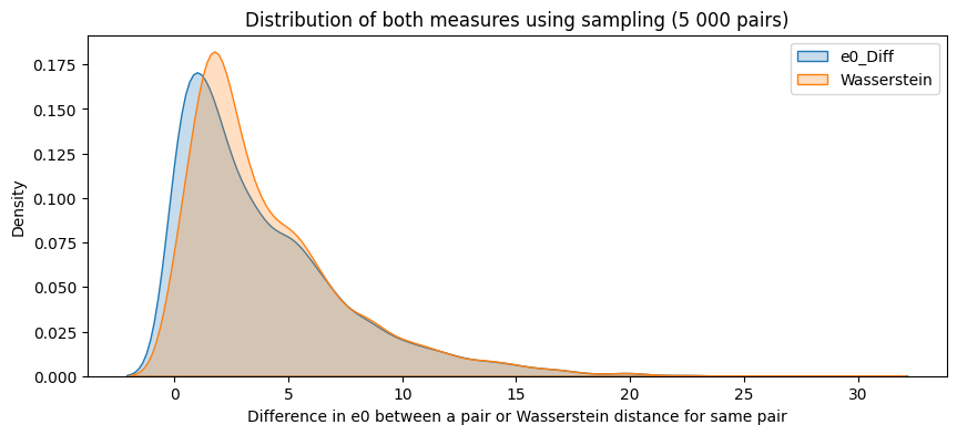
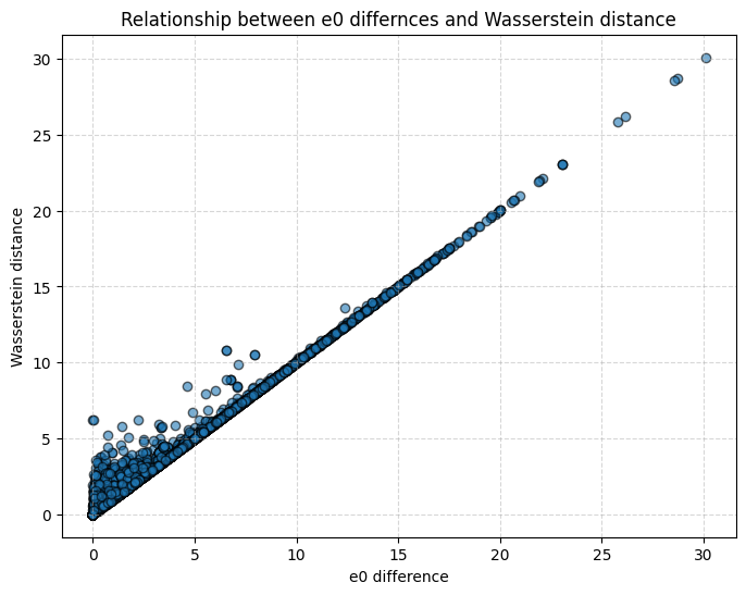
Calculating the two measures for all available pairs would take way too much time as they are many possible combinations (13 700 when considering only one gender). Instead, the following code will sample from the data. That is, it will generate random pairs. Here, I focus only on data for both sexes combined. I sample 5 000 pairs from the data.
df_both = HMD_LTs[HMD_LTs["Sex"] == "Both"]
years = df_both["Year"].unique()

years = df_both["Year"].unique()
countries = df_both["Country"].unique()

num_pairs = len(years) * len(countries)
print(f"Total possible year-country combinations: {num_pairs}")
#Total possible year-country combinations: 13700

results = []
pairs_sampled = 0
max_samples = 5000

while pairs_sampled < max_samples:

    year = random.choice(years)
    countries = df_both[df_both["Year"] == year]["Country"].unique()

    if len(countries) < 2:
        continue

    c1, c2 = random.sample(list(countries), 2)

    res = get_comparison_for_pair(HMD_LTs, year, "Both", c1, c2)

    if res is not None:
        results.append(res)
        pairs_sampled += 1

final_df = pd.DataFrame(results)
final_df.head()

import seaborn as sns
import matplotlib.pyplot as plt

plt.figure(figsize=(10,4))

sns.kdeplot(final_df["e0_Diff"], label="e0_Diff", fill=True)
sns.kdeplot(final_df["Wasserstein"], label="Wasserstein", fill=True)

plt.title(f"Distribution of both measures using sampling (5 000 pairs)")
plt.xlabel("Difference in e0 between a pair or Wasserstein distance for same pair")
plt.legend()
plt.show()
plt.figure(figsize=(8, 6))
plt.scatter(final_df["e0_Diff"], final_df["Wasserstein"], alpha=0.6, edgecolor="k")
plt.xlabel("e0 difference")
plt.ylabel("Wasserstein distance")
plt.title("Relationship between e0 differnces and Wasserstein distance")
plt.grid(True, linestyle="--", alpha=0.5)
plt.show()
from scipy.stats import pearsonr
r, p_value = pearsonr(final_df["e0_Diff"], final_df["Wasserstein"])

print(f"Pearson r: {r:.3f}")
print(f"P-value: {p_value:.3e}")
#Pearson r: 0.991
#P-value: 0.000e+00

# Compute Pearson's r
r_kl, _ = pearsonr(final_df["Wasserstein"], final_df["KL_divergence"])
r_jaccard, _ = pearsonr(final_df["Wasserstein"], final_df["Jaccard_distance"])

# plot
fig, axes = plt.subplots(1, 2, figsize=(14, 6), sharex=False, sharey=False)

axes[0].scatter(final_df["Wasserstein"], final_df["KL_divergence"],
                alpha=0.6, edgecolor="k")
axes[0].set_xlabel("Wasserstein distance")
axes[0].set_ylabel("Kullback–Leibler divergence")
axes[0].set_title("KL divergence vs. Wasserstein")
axes[0].grid(True, linestyle="--", alpha=0.5)
axes[0].text(0.05, 0.95, f"r = {r_kl:.2f}",
             transform=axes[0].transAxes, fontsize=12,
             verticalalignment="top", bbox=dict(boxstyle="round", facecolor="white", alpha=0.7))

axes[1].scatter(final_df["Wasserstein"], final_df["Jaccard_distance"],
                alpha=0.6, edgecolor="k", color="tab:orange")
axes[1].set_xlabel("Wasserstein distance")
axes[1].set_ylabel("Jaccard distance")
axes[1].set_title("Jaccard distance vs. Wasserstein")
axes[1].grid(True, linestyle="--", alpha=0.5)
axes[1].text(0.05, 0.95, f"r = {r_jaccard:.2f}",
             transform=axes[1].transAxes, fontsize=12,
             verticalalignment="top", bbox=dict(boxstyle="round", facecolor="white", alpha=0.7))

plt.tight_layout()
plt.show()
Find the most interesting cases
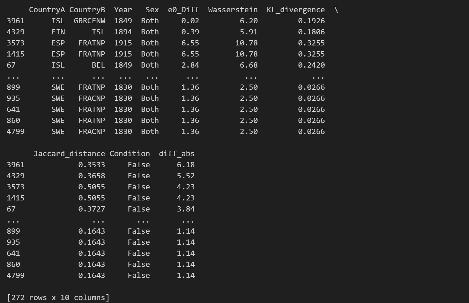
In which pairs is the gap between \(e_0\) differences and Wasserstein distance particulary large? What is the highest Wasserstein distance observed in the data? Where is the gap in \(e_0\) largest and does the Wasserstein distance suggest large differences in the age-at-death distribution as well?
final_df["diff_abs"] = (final_df["e0_Diff"] - final_df["Wasserstein"]).abs()
threshold = final_df["diff_abs"].quantile(0.95)

interesting_cases = final_df[final_df["diff_abs"] >= threshold]
df_sorted = interesting_cases.sort_values(by='diff_abs', ascending=False)
print(df_sorted)
df_sorted2 = final_df.sort_values(by="Wasserstein", ascending=False)
df_sorted2.head()

df_sorted3 = final_df.sort_values(by="e0_Diff", ascending=False)
df_sorted3.head()

Plot the most interesting cases
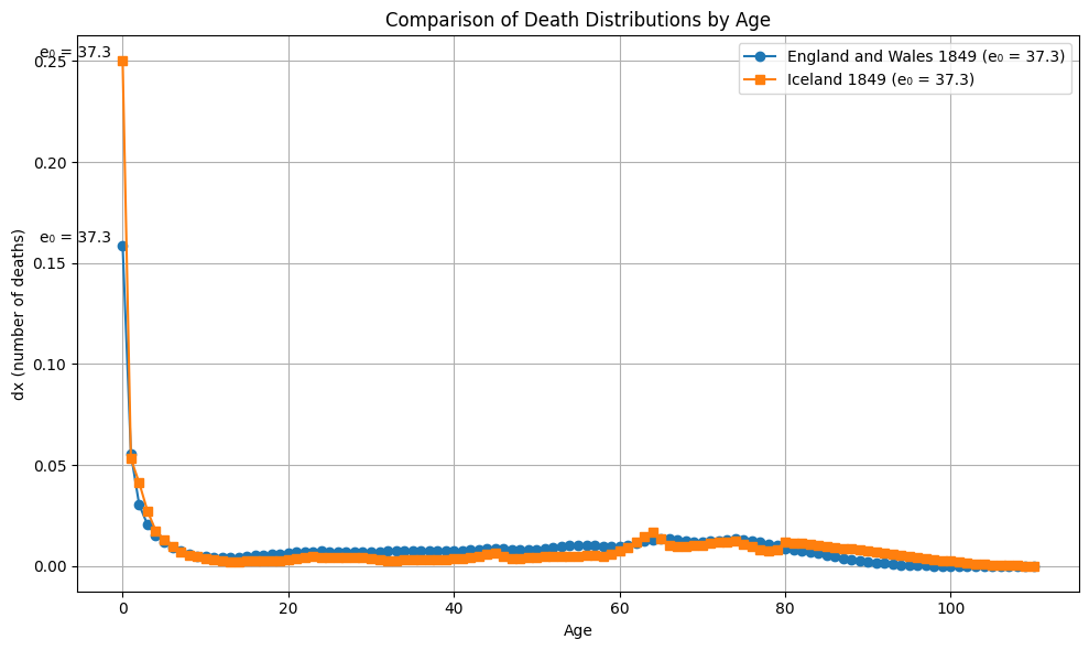
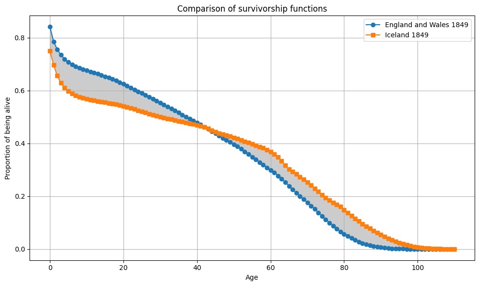
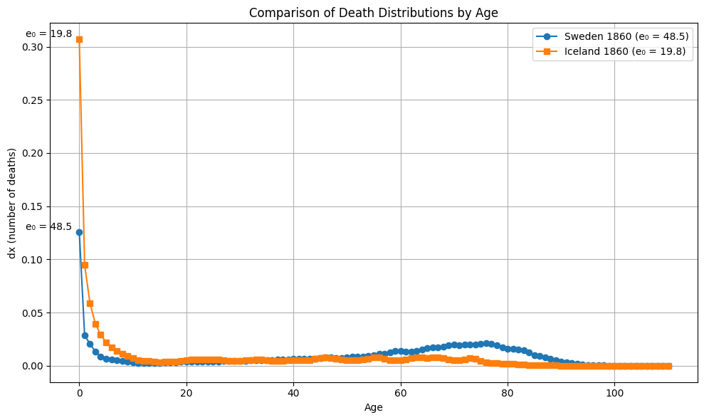
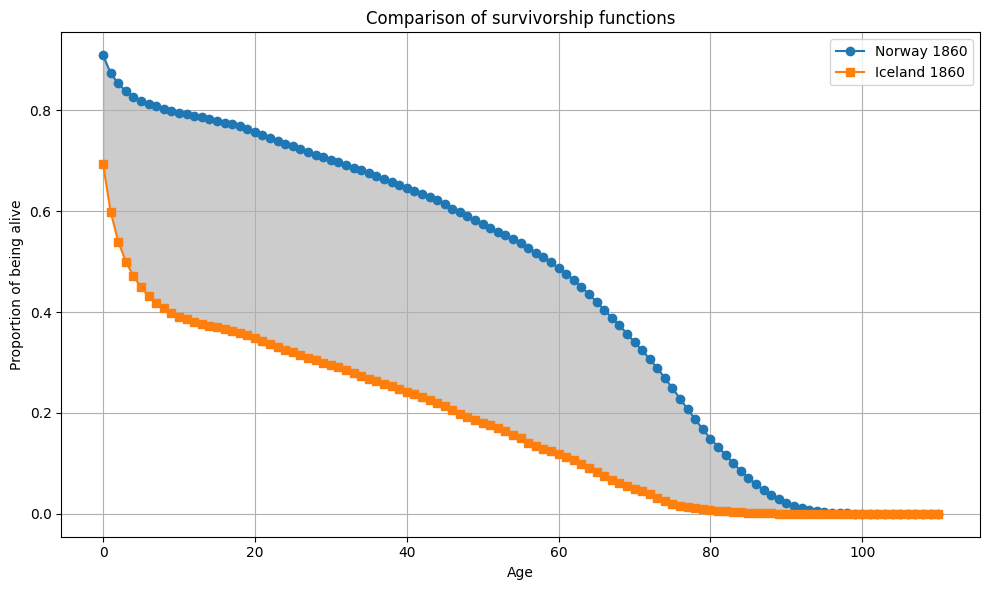
From all 10 000 samples, the largest gap between \(e_0\) differences and Wasserstein distance is observed between Iceland and England and Wales in 1849 (6.2). The largest Wasserstein distance is observed between Sweden and Iceland in 1860 with 28.6. This is also the pair with the largest gap in \(e_0\) in this sample.
def get_dx_for_plot(df, year):
    qx = df.loc[df["Year"] == year, "qx"].values
    lx = np.concatenate(([1], np.cumprod(1 - qx)[:-1]))
    dx = np.concatenate((-np.diff(lx), [lx[-1]]))
    return dx

def get_e0_for_plot(df, year):
    ex = df.loc[df["Year"] == year, "ex"].values
    e0 = ex[0]
    return e0

def get_Sx_for_plot(dx):
    CDF = np.cumsum(dx)
    Sx = 1 - CDF
    return Sx

def plot_dx(ages, dx1, dx2, e0_1, e0_2, label1, label2):
    plt.figure(figsize=(10, 6))
    plt.plot(ages, dx1, label=f"{label1} (e₀ = {e0_1:.1f})", marker='o')
    plt.plot(ages, dx2, label=f"{label2} (e₀ = {e0_2:.1f})", marker='s')
    plt.text(ages[np.argmax(dx1)]-10, max(dx1), f"e₀ = {e0_1:.1f}", fontsize=10, ha='left', va='bottom')
    plt.text(ages[np.argmax(dx2)]-10, max(dx2), f"e₀ = {e0_2:.1f}", fontsize=10, ha='left', va='bottom')
    plt.title("Comparison of Death Distributions by Age")
    plt.xlabel("Age")
    plt.ylabel("dx (number of deaths)")
    plt.legend()
    plt.grid(True)
    plt.tight_layout()
    plt.show()

def plot_Sx(ages, Sx1, Sx2, label1, label2):
    plt.figure(figsize=(10, 6))
    plt.plot(ages, Sx1, label=f"{label1}", marker='o')
    plt.plot(ages, Sx2, label=f"{label2}", marker='s')
    plt.fill_between(ages, Sx1, Sx2, color='gray', alpha=0.4)
    plt.title("Comparison of survivorship functions")
    plt.xlabel("Age")
    plt.ylabel("Proportion of being alive")
    plt.legend()
    plt.grid(True)
    plt.tight_layout()
    plt.show()

# plot first interesting case
the_year = 1849

pair1 = HMD_LTs[(HMD_LTs['Year'] == the_year) &
               (HMD_LTs['Sex'] == "Both") &
               (HMD_LTs['Country'] == "GBRTENW")]

dx1 = get_dx_for_plot(pair1, the_year)
e0_1 = get_e0_for_plot(pair1, the_year)

pair2 = HMD_LTs[(HMD_LTs['Year'] == the_year) &
               (HMD_LTs['Sex'] == "Both") &
               (HMD_LTs['Country'] == "ISL")]

dx2 = get_dx_for_plot(pair2, the_year)
e0_2 = get_e0_for_plot(pair2, the_year)

Sx1 = get_Sx_for_plot(dx1)
Sx2 = get_Sx_for_plot(dx2)

ages = np.arange(len(dx1))

plot_dx(ages, dx1, dx2, e0_1, e0_2, "England and Wales 1849", "Iceland 1849")
plot_Sx(ages, Sx1, Sx2, "England and Wales 1849", "Iceland 1849")
# plot second interesting case
the_year = 1860

pair1 = HMD_LTs[(HMD_LTs['Year'] == the_year) &
               (HMD_LTs['Sex'] == "Both") &
               (HMD_LTs['Country'] == "SWE")]

dx1 = get_dx_for_plot(pair1, the_year)
e0_1 = get_e0_for_plot(pair1, the_year)

pair2 = HMD_LTs[(HMD_LTs['Year'] == the_year) &
               (HMD_LTs['Sex'] == "Both") &
               (HMD_LTs['Country'] == "ISL")]

dx2 = get_dx_for_plot(pair2, the_year)
e0_2 = get_e0_for_plot(pair2, the_year)

Sx1 = get_Sx_for_plot(dx1)
Sx2 = get_Sx_for_plot(dx2)

plot_dx(ages, dx1, dx2, e0_1, e0_2, "Sweden 1860", "Iceland 1860")
plot_Sx(ages, Sx1, Sx2, "Sweden 1860", "Iceland 1860")
Second analysis: What about more recent years?
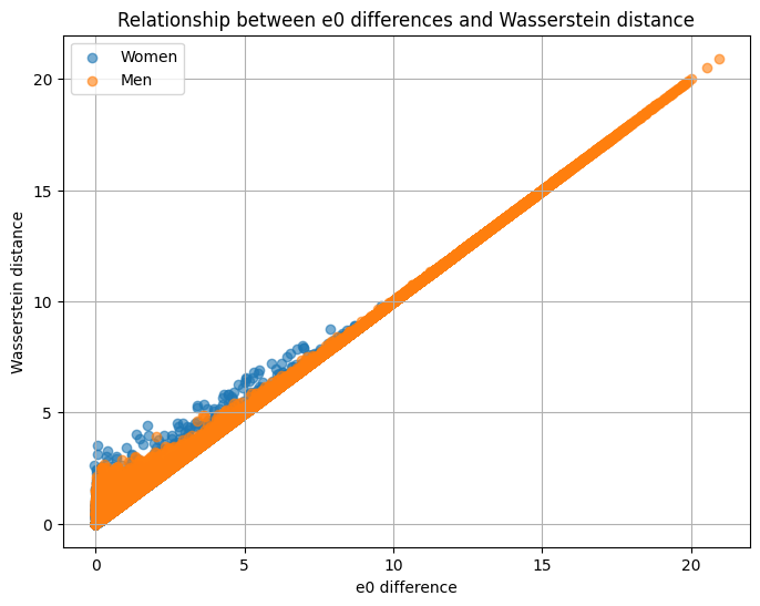
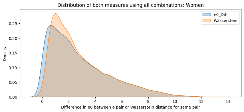
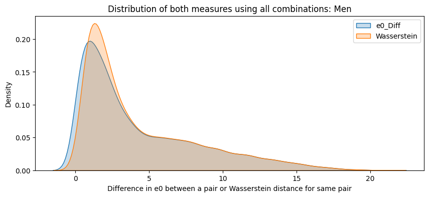
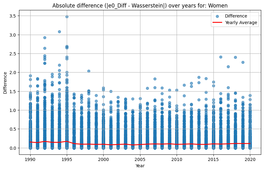
Let’s focus only on the last decades and examine the relationship observed between 1990 and 2020. This time we do not sample but calculate all possible combinations.
def get_comparison(HMD_LTs, year, sex):
    subset_df = HMD_LTs[(HMD_LTs["Sex"] == sex) & (HMD_LTs["Year"] == year)].copy()
    countries = subset_df["Country"].unique()

    # Store dx (age-at-death distributions)
    dx_dict = {}
    for country in countries:
        country_df = subset_df[subset_df["Country"] == country]
        if country_df.empty:
            continue
        dx_dict[country] = get_dx(country_df)

    # All country pairs
    country_pairs = list(itertools.combinations(countries, 2))

    results = []
    for c1, c2 in country_pairs:
        val1 = subset_df.loc[subset_df["Country"] == c1, "ex"].iloc[0]
        val2 = subset_df.loc[subset_df["Country"] == c2, "ex"].iloc[0]

        # Define CountryA (higher life expectancy) and CountryB
        if val1 >= val2:
            countryA, countryB = c1, c2
        else:
            countryA, countryB = c2, c1

        dx1 = dx_dict[countryA]
        dx2 = dx_dict[countryB]

        # Get survival functions
        Sx1 = 1 - np.cumsum(dx1)
        Sx2 = 1 - np.cumsum(dx2)

        # Condition check
        condition = "True" if np.all(Sx1 >= Sx2) else "False"

        # Distances
        Wasserstein = np.sum(np.abs(Sx1 - Sx2))
        e0_diff = np.sum(Sx1 - Sx2)
        KL_divergence = get_KL_divergence(dx1, dx2)
        Jaccard_distance = get_Jaccard_distance(dx1, dx2)

        results.append({
            "CountryA": countryA,
            "CountryB": countryB,
            "Year": year,
            "Sex": sex,
            "e0_Diff": round(e0_diff, 2),
            "Wasserstein": round(Wasserstein, 2),
            "KL_divergence": round(KL_divergence, 4),
            "Jaccard_distance": round(Jaccard_distance, 4),
            "Condition": condition
        })

    diff_df = pd.DataFrame(results)
    return diff_df

#get all combinations for women and men, separatly
all_results = []

for sex in ["Women", "Men"]:
    for year in range(1990, 2021):
        df_diff = get_comparison(HMD_LTs, year, sex)
        if df_diff is not None and not df_diff.empty:
            all_results.append(df_diff)

final_df = pd.concat(all_results, ignore_index=True)

# plot the relationship
plt.figure(figsize=(8,6))
for sex, color in zip(["Women", "Men"], ["blue", "red"]):
    subset = final_df[final_df["Sex"] == sex]
    plt.scatter(subset["e0_Diff"], subset["Wasserstein"], alpha=0.6, label=sex)

plt.xlabel("e0 difference")
plt.ylabel("Wasserstein distance")
plt.title("Relationship between e0 differences and Wasserstein distance")
plt.legend()
plt.grid(True)
plt.show()
for sex in ["Women", "Men"]:
    subset = final_df[final_df["Sex"] == sex]
    plt.figure(figsize=(10,4))

    sns.kdeplot(subset["e0_Diff"], label="e0_Diff", fill=True)
    sns.kdeplot(subset["Wasserstein"], label="Wasserstein", fill=True)

    plt.title(f"Distribution of both measures using all combinations: {sex}")
    plt.xlabel("Difference in e0 between a pair or Wasserstein distance for same pair")
    plt.legend()
    plt.show()
final_df["e0_Diff"] = pd.to_numeric(final_df["e0_Diff"], errors='coerce')
final_df["Wasserstein"] = pd.to_numeric(final_df["Wasserstein"], errors='coerce')

final_df["Diff_e0_Wasserstein"] = abs(final_df["e0_Diff"] - final_df["Wasserstein"])

for sex in ["Women", "Men"]:
    df_sex = final_df[final_df["Sex"] == sex]

    yearly_avg = df_sex.groupby("Year")["Diff_e0_Wasserstein"].mean().reset_index()

    plt.figure(figsize=(10, 6))
    plt.scatter(df_sex["Year"], df_sex["Diff_e0_Wasserstein"], alpha=0.6, label="Difference")
    plt.plot(yearly_avg["Year"], yearly_avg["Diff_e0_Wasserstein"], color="red", linewidth=2, label="Yearly Average")
    plt.title(f"Absolute difference (|e0_Diff - Wasserstein|) over years for: {sex}")
    plt.xlabel("Year")
    plt.ylabel("Difference")
    plt.grid(True)
    plt.legend()
    plt.show()
for sex in ["Women", "Men"]:
    df_sex = final_df[final_df["Sex"] == sex]
    if df_sex.empty:
        continue

    # Pearson correlations
    r_kl, _ = pearsonr(df_sex["Wasserstein"], df_sex["KL_divergence"])
    r_jaccard, _ = pearsonr(df_sex["Wasserstein"], df_sex["Jaccard_distance"])

    fig, axes = plt.subplots(1, 2, figsize=(14, 6))

    axes[0].scatter(df_sex["Wasserstein"], df_sex["KL_divergence"],
                    alpha=0.6, edgecolor="k")
    axes[0].set_xlabel("Wasserstein distance")
    axes[0].set_ylabel("Kullback–Leibler divergence")
    axes[0].set_title(f"{sex}: KL vs. Wasserstein")
    axes[0].grid(True, linestyle="--", alpha=0.5)
    axes[0].text(0.05, 0.95, f"r = {r_kl:.2f}",
                 transform=axes[0].transAxes,
                 fontsize=12, verticalalignment="top",
                 bbox=dict(boxstyle="round", facecolor="white", alpha=0.7))

    axes[1].scatter(df_sex["Wasserstein"], df_sex["Jaccard_distance"],
                    alpha=0.6, edgecolor="k", color="tab:orange")
    axes[1].set_xlabel("Wasserstein distance")
    axes[1].set_ylabel("Jaccard distance")
    axes[1].set_title(f"{sex}: Jaccard vs. Wasserstein")
    axes[1].grid(True, linestyle="--", alpha=0.5)
    axes[1].text(0.05, 0.95, f"r = {r_jaccard:.2f}",
                 transform=axes[1].transAxes,
                 fontsize=12, verticalalignment="top",
                 bbox=dict(boxstyle="round", facecolor="white", alpha=0.7))

    plt.tight_layout()
    plt.show()
Third analysis: Investigating sex differences in mortality using the Wasserstein distance
Since women usually outlive men it might be interesting to compare differences between women and men on the basis of the Wasserstein distance.
def get_comparison_sex_diff(HMD_LTs, year):
    subset_df = HMD_LTs[HMD_LTs["Year"] == year].copy()
    countries = subset_df["Country"].unique()
    results = []

    for country in countries:
        women_df = subset_df[(subset_df["Country"] == country) & (subset_df["Sex"] == "Women")]
        men_df = subset_df[(subset_df["Country"] == country) & (subset_df["Sex"] == "Men")]

        if women_df.empty or men_df.empty:
            continue

        # Get dx distributions
        dx_women = get_dx(women_df)
        dx_men = get_dx(men_df)

        # Survival functions (needed for Wasserstein + condition)
        Sx_women = 1 - np.cumsum(dx_women)
        Sx_men = 1 - np.cumsum(dx_men)

        # Condition check
        condition = "True" if np.all(Sx_women >= Sx_men) else "False"

        # Distances
        e0_diff = np.sum(Sx_women - Sx_men)
        wasserstein = np.sum(np.abs(Sx_women - Sx_men))
        KL_divergence = get_KL_divergence(dx_women, dx_men)
        Jaccard_distance = get_Jaccard_distance(dx_women, dx_men)

        results.append({
            "Country": country,
            "Year": year,
            "e0_Diff": round(e0_diff, 2),
            "Wasserstein": round(wasserstein, 2),
            "KL_divergence": round(KL_divergence, 4),
            "Jaccard_distance": round(Jaccard_distance, 4),
            "Condition": condition
        })

    diff_df = pd.DataFrame(results)
    return diff_df

# loop over years
all_results_sex_diff = []

for year in range(1990, 2021):
    df_diff = get_comparison_sex_diff(HMD_LTs, year)
    if df_diff is not None and not df_diff.empty:
        all_results_sex_diff.append(df_diff)

final_df_sex_diff = pd.concat(all_results_sex_diff, ignore_index=True)

r, p_value = pearsonr(final_df_sex_diff["e0_Diff"], final_df_sex_diff["Wasserstein"])

print(f"Pearson r: {r:.3f}")
print(f"P-value: {p_value:.3e}")
#Pearson r: 1.000
#P-value: 0.000e+00

# plot the differences
final_df_sex_diff["Diff_e0_Wasserstein"] = abs(final_df_sex_diff["e0_Diff"] - final_df_sex_diff["Wasserstein"])
yearly_avg = final_df_sex_diff.groupby("Year")["Diff_e0_Wasserstein"].mean().reset_index()

plt.figure(figsize=(10,6))
plt.scatter(final_df_sex_diff["Year"], final_df_sex_diff["Diff_e0_Wasserstein"], alpha=0.6)
plt.plot(yearly_avg["Year"], yearly_avg["Diff_e0_Wasserstein"], color="red", linewidth=2, label="Yearly Average")
plt.title("Difference (|e0 difference - Wasserstein|) over time, focusing on sex differences only")
plt.xlabel("Year")
plt.ylabel("Difference (|e0 difference - Wasserstein distance|)")
plt.grid(True)
plt.show()
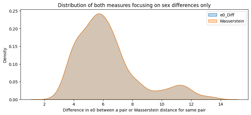
plt.figure(figsize=(10,4))

sns.kdeplot(final_df_sex_diff["e0_Diff"], label="e0_Diff", fill=True)
sns.kdeplot(final_df_sex_diff["Wasserstein"], label="Wasserstein", fill=True)

plt.title(f"Distribution of both measures focusing on sex differences only")
plt.xlabel("Difference in e0 between a pair or Wasserstein distance for same pair")
plt.legend()
plt.show()
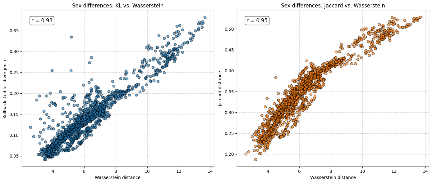
r_kl, _ = pearsonr(final_df_sex_diff["Wasserstein"], final_df_sex_diff["KL_divergence"])
r_jaccard, _ = pearsonr(final_df_sex_diff["Wasserstein"], final_df_sex_diff["Jaccard_distance"])

fig, axes = plt.subplots(1, 2, figsize=(14, 6))

axes[0].scatter(final_df_sex_diff["Wasserstein"], final_df_sex_diff["KL_divergence"],
                alpha=0.6, edgecolor="k")
axes[0].set_xlabel("Wasserstein distance")
axes[0].set_ylabel("Kullback–Leibler divergence")
axes[0].set_title("Sex differences: KL vs. Wasserstein")
axes[0].grid(True, linestyle="--", alpha=0.5)
axes[0].text(0.05, 0.95, f"r = {r_kl:.2f}",
             transform=axes[0].transAxes, fontsize=12,
             verticalalignment="top",
             bbox=dict(boxstyle="round", facecolor="white", alpha=0.7))

axes[1].scatter(final_df_sex_diff["Wasserstein"], final_df_sex_diff["Jaccard_distance"],
                alpha=0.6, edgecolor="k", color="tab:orange")
axes[1].set_xlabel("Wasserstein distance")
axes[1].set_ylabel("Jaccard distance")
axes[1].set_title("Sex differences: Jaccard vs. Wasserstein")
axes[1].grid(True, linestyle="--", alpha=0.5)
axes[1].text(0.05, 0.95, f"r = {r_jaccard:.2f}",
             transform=axes[1].transAxes, fontsize=12,
             verticalalignment="top",
             bbox=dict(boxstyle="round", facecolor="white", alpha=0.7))

plt.tight_layout()
plt.show()
Conclusions
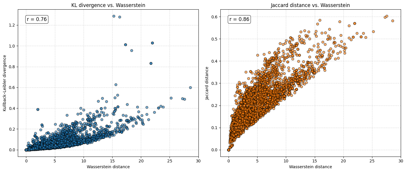
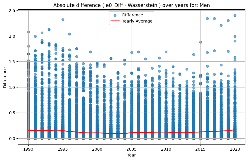
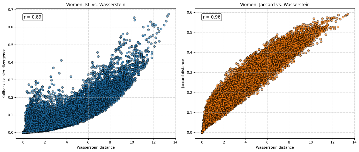
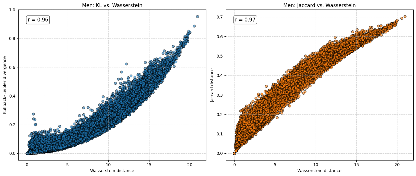
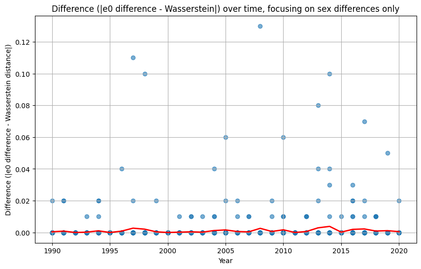
The analysis suggests that the difference in \(e_0\) is often very similar to the Wasserstein distance. This indicates that the difference in the mean age at death can be interpreted as distributional differences in most cases. We do find examples where both measures do not correspond to each other at all. For instance, England and Wales shows a very similar mean age at death (or life expectancy at birth) to Iceland in the year 1849. Yet, the Wasserstein distance suggests that the age-at-death distributions differ substantially from each other. It’s value is about 6, while the Wasserstein distance is on average about 4. Theoretically, the Wasserstein distance can be 110 because we are looking at single ages from 0 to 110+. The reason for the deviation between \(e_0\) differences and the Wasserstein distance is the particulary large infant mortality in Iceland with lower mortality at older ages. For more recent years and especially when comparing the mortality of women and men, differences in \(e_0\) and the Wasserstein distance correspond to each other very strongly (the yearly difference in both measures is on average below 0.5 and for sex differences in mortality even close to 0.0). Finally, the results indicate that there is a strong correlation between the Wasserstein distance and the non-overlap index (Jaccard index) as well as between the Wasserstein distance and the KL-divergence. In other words, the three measures evaluate distributional differences very similar.
Notebook
The jupyter notebook can be found here: https://github.com/msauerberg/msauerberg.github.io/blob/main/assets/jupyter/Wasserstein_HMD_analysis.ipynb.
Paper
The paper can be found here: https://arxiv.org/abs/2508.17235.
@misc{sauerberg2025,
  title={On the relationship between the Wasserstein distance and differences in life expectancy at birth},
  author={Markus Sauerberg},
  year={2025},
  eprint={2508.17235},
  archivePrefix={arXiv},
  primaryClass={stat.AP},
  url={https://arxiv.org/abs/2508.17235},
}
Enjoy Reading This Article?
Here are some more articles you might like to read next: