Short description of the Wasserstein distance

The Wasserstein distance (or earth mover’s distance) computes the minimum “work” needed to transform one distribution into the other and refers to optimal transport theory. According to https://docs.scipy.org, the Wasserstein distance “is a similarity metric between two probability distributions. In the discrete case, the Wasserstein distance can be understood as the cost of an optimal transport plan to convert one distribution into the other. The cost is calculated as the product of the amount of probability mass being moved and the distance it is being moved.”

In the one-dimensional case and when the cost function is defined as,

the Wasserstein distance can be expressed as,

\begin{equation} W(u,v)=\int_{-\infty}^{\infty}|U-V|, \end{equation}

where \(U\) and \(V\) are the respective cumulative distribution functions (CDF) of \(u\) and \(v\). See Santambrogio (2015), chapter 2 for more details Santambrogio (2015).

Short description of life expectancy at birth

In demography, life expectancy at birth (\(e_0\)) measures the expected number of life years on the basis of a set of age-specific mortality rates. \(e_0\) is derived from a period life table - a procedure where age-specific mortality rates are applied to hypothetical cohort to calculate the number of persons alive and deceased in each age interval. This table will then be used to derive the expected number of life years. Usually, the size of the initial life table population is set to 100 000 persons. The number of deceased persons in each age interval is denoted as \(d_x\), while \(l_x\) gives the age-specific number of persons alive. When setting the initial size of the life table population to \(1\), the \(d_x\) function can be seen as a probability density function (PDF). \(e_0\) is the mean age at death,

\begin{equation} e_0=\frac{\int_0^{\omega}x\cdot d(x)dx}{\int_0^{\omega}d(x)dx}, \end{equation}

where $\omega$ denotes the upper age interval. A more popular formular, however, is expressing \(e_0\) as the area under the survivorship curve,

\begin{equation} e_0=\int_0^{\omega}l(x)dx. \end{equation}

The difference between two \(e_0\) values is then,

\begin{equation} e_{0,A}-e_{0,B} = \int_0^{\omega}(l_A(x)-l_B(x))dx \end{equation}

The relationship between the Wasserstein distance and difference between two life expectancy at birth values

It is well-known in surival analysis that PDF, CDF, and the survivorship function are directly linked to each other. That is, the survivorship function can be derived from the PDF and is complement of the CDF,

As shown above, the Wasserstein distance is the area between two CDFs. Substituting the CDFs with the life table survivorship function \(l_x\) gives,

\begin{equation} W(d_A,d_B)=\int_{0}^{\omega}|l_A(x)-l_B(x)|dx. \end{equation}

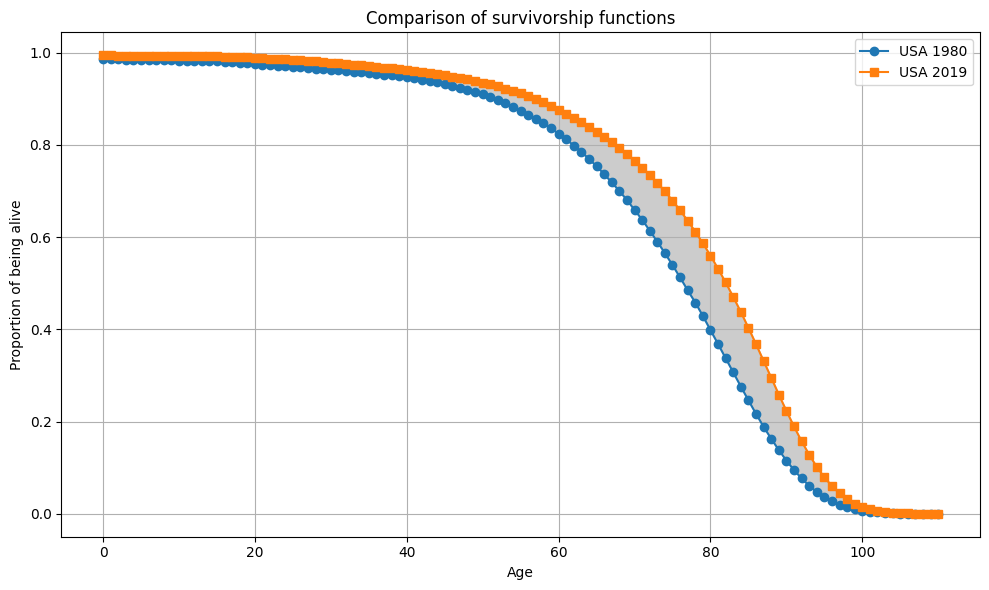
This implies that the difference between two \(e_0\) values is equal to the Wasserstein distance between two life table age-at-death distributions, whenever \(l_A(x) >= l_B(x)\) for all \(x\).

Calculations

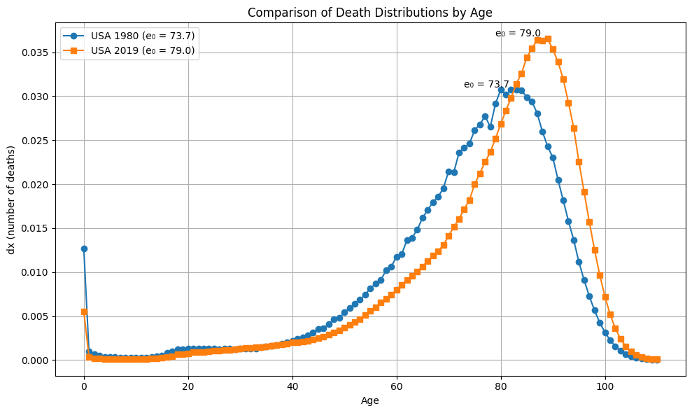
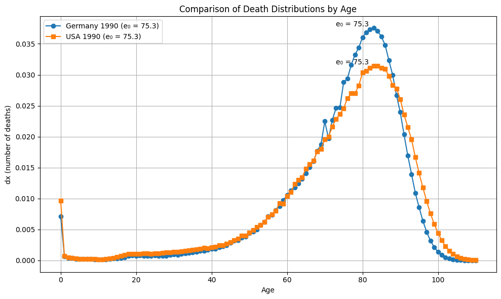
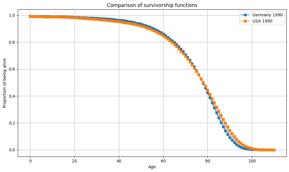
The first example demonstrates the case where the Wasserstein distance correponds to the difference in \(e_0\), while the second one shows that the difference in \(e_0\) can be very small even though the age-at-death distributions differ substantially from each other. This is captured by the Wasserstein distance correctly.

Demonstration in Python using life tables from the Human Mortality Database

import pandas as pd
import numpy as np
import matplotlib.pyplot as plt
from scipy.stats import wasserstein_distance

#Data can be downloaded from https://mortality.org/
USA = pd.read_csv("bltper_1x1_US.txt", sep="\s+", skiprows=2)
Germany = pd.read_csv("bltper_1x1_Germany.txt", sep="\s+", skiprows=2)

# Please note that I use "lx" and "Sx" interchangeable for denoting the survivorship function.

def get_dx(df, year):
    qx = df.loc[df["Year"] == year, "qx"].values
    lx = np.concatenate(([1], np.cumprod(1 - qx)[:-1]))
    dx = np.concatenate((-np.diff(lx), [lx[-1]]))
    return dx

def get_e0(df, year):
    ex = df.loc[df["Year"] == year, "ex"].values
    e0 = ex[0]
    return e0

def plot_dx(ages, dx1, dx2, e0_1, e0_2, label1, label2):
    plt.figure(figsize=(10, 6))
    plt.plot(ages, dx1, label=f"{label1} (e₀ = {e0_1:.1f})", marker='o')
    plt.plot(ages, dx2, label=f"{label2} (e₀ = {e0_2:.1f})", marker='s')
    plt.text(ages[np.argmax(dx1)]-10, max(dx1), f"e₀ = {e0_1:.1f}", fontsize=10, ha='left', va='bottom')
    plt.text(ages[np.argmax(dx2)]-10, max(dx2), f"e₀ = {e0_2:.1f}", fontsize=10, ha='left', va='bottom')
    plt.title("Comparison of Death Distributions by Age")
    plt.xlabel("Age")
    plt.ylabel("dx (number of deaths)")
    plt.legend()
    plt.grid(True)
    plt.tight_layout()
    plt.show()

def plot_Sx(ages, Sx1, Sx2, label1, label2):
    plt.figure(figsize=(10, 6))
    plt.plot(ages, Sx1, label=f"{label1}", marker='o')
    plt.plot(ages, Sx2, label=f"{label2}", marker='s')
    plt.fill_between(ages, Sx1, Sx2, color='gray', alpha=0.4)
    plt.title("Comparison of survivorship functions")
    plt.xlabel("Age")
    plt.ylabel("Proportion of being alive")
    plt.legend()
    plt.grid(True)
    plt.tight_layout()
    plt.show()

def get_Sx(dx):
    CDF = np.cumsum(dx)
    Sx = 1 - CDF
    return Sx

def get_Wasserstein(dx1, dx2):
    CDF1 = np.cumsum(dx1)
    Sx1 = 1 - CDF1
    CDF2 = np.cumsum(dx2)
    Sx2 = 1 - CDF2
    Sx_diff_absolute = abs(Sx1 - Sx2)
    Wasserstein = round(np.sum(Sx_diff_absolute), 2)
    return Wasserstein  

dx_1980_US = get_dx(USA, 1980)
dx_1990_US = get_dx(USA, 1990)
dx_2019_US = get_dx(USA, 2019)

ages = np.arange(len(dx_1980_US))

dx_1990_Germany = get_dx(Germany, 1990)

e0_1980_US = get_e0(USA, 1980)
e0_1990_US = get_e0(USA, 1990)
e0_2019_US = get_e0(USA, 2019)
e0_1990_Germany = get_e0(Germany, 1990)

Sx_1980_US = get_Sx(dx_1980_US)
Sx_1990_US = get_Sx(dx_1990_US)
Sx_2019_US = get_Sx(dx_2019_US)
Sx_1990_Germany = get_Sx(dx_1990_Germany)

plot_dx(ages, dx_1980_US, dx_2019_US, e0_1980_US, e0_2019_US, "USA 1980", "USA 2019")
plot_Sx(ages, Sx_1980_US, Sx_2019_US, "USA 1980", "USA 2019")

condition = np.all(Sx_2019_US >= Sx_1980_US)
if condition:
    print("Sx1 >= Sx2 for all x")
else:
    print("Sx1 not always >= Sx2 for all x")



Difference_in_e0_US_2019_and_US_1980 = round(e0_2019_US - e0_1980_US, 2)
Wasserstein_between_2019_US_1980_US = get_Wasserstein(dx_2019_US, dx_1980_US)
Wasserstein_scipy = round(wasserstein_distance(ages, ages, dx_2019_US, dx_1980_US), 2)

print(f"The difference in e0 is: {Difference_in_e0_US_2019_and_US_1980}")
print(f"The Wasserstein distance is: {Wasserstein_between_2019_US_1980_US}")
print(f"The Wasserstein distance from Scipy: {Wasserstein_scipy}")

#Sx1 >= Sx2 for all x
#The difference in e0 is: 5.21
#The Wasserstein distance is: 5.21
#The Wasserstein distance from Scipy: 5.21

plot_dx(ages, dx_1990_Germany, dx_1990_US, e0_1990_Germany, e0_1990_Germany, "Germany 1990", "USA 1990")
plot_Sx(ages, Sx_1980_US, Sx_2019_US, "Germany 1990", "USA 1990")

condition = np.all(Sx_1990_Germany >= Sx_1990_US)
if condition:
    print("Sx1 >= Sx2 for all x")
else:
    print("Sx1 not always >= Sx2 for all x")

Difference_in_e0_Germany_1990_and_US_1990 = round(e0_1990_Germany - e0_1990_US, 2)
Wasserstein_between_Germany_1990_US_1990_US = get_Wasserstein(dx_1990_Germany, dx_1990_US)
Wasserstein_scipy = round(wasserstein_distance(ages, ages, dx_1990_Germany, dx_1990_US), 2)

print(f"The difference in e0 is: {Difference_in_e0_Germany_1990_and_US_1990}")
print(f"The Wasserstein distance is: {Wasserstein_between_Germany_1990_US_1990_US}")
print(f"The Wasserstein distance from Scipy is: {Wasserstein_scipy}")

#Sx1 not always >= Sx2 for all x
#The difference in e0 is: -0.05
#The Wasserstein distance is: 1.56
#The Wasserstein distance from Scipy is: 1.56

Conclusion

When the survivorship functions between two populations do not crossover, the Wasserstein distance is equal to the difference in \(e_0\). Hence, we do not compare the means of two age-at death distibutions anymore - as usually when comparing two \(e_0\) values - but we solve the optimal transport problem. This offers a novel interpretation to \(e_0\) differences. There are also cases where the two measures do not correspond to each other. For instance, between the US and Germany in 1990, the difference in \(e_0\) suggests rather small mortality differences between the two populationss. The Wasserstein distance captures those differences between the two age-at death distributions better as it reflects the absolute difference between the survivorship functions. In contrast, differences in \(e_0\) are more “net differences” in survivorship because positive and negative difference in \(l(x)\) can cancel each other out. This makes sense when the aim is examining the differences in the expected number of life years. It does not, however, give us a good sense of how different the underlying age-at-death distributions actually are. For this reason, it makes sense to calculate both measures. In cases where both measures gives similar results, the difference in \(e_0\) reflects not only differences in the mean age at death but takes into account all distributional differences. This might be the case for comparing women and men in most countries becaue men usually show higher death rates at all ages. For those cases where the Wasserstein distance and the difference in \(e_0\) differ, it might be worthwhile investigating the age-at-death distributions more closely. Obviously, there are other measures such as the standard deviation or interquartile range that provide information on distributional differences. Yet, the calculation of the Wasserstein distance is very similar to deriving differences in \(e_0\) plus, more importantly, the Wasserstein distance offers a fancy way to think about distributions than the standard approaches :-) Thanks for reading!

Notebook

The jupyter notebook can be found here: https://github.com/msauerberg/msauerberg.github.io/blob/main/assets/jupyter/wasserstein.ipynb.